May 19, 2019
Get formatted versions: Word : PDF
Orientation
As you’ve probably figured out already, the columns of data frames are called variables because the values in the column are not all the same, that is, they vary.
In the early 1800s, it was discovered that many different variables have a pattern in common: the most common values are near the mean and values become less common the further they are from the mean. Not all variables have this pattern, but many do and so the pattern came to be called the normal distribution.
In this lesson, you’re going to look at several different variables and compare them to the normal distribution. Based on this comparison, you’ll be able to make an appropriate description in words of the distribution.
Here are three rules of thumb, each of which can be used to estimate the mean and standard deviation of a distribution:
Mark off the interval containing the center two-thirds of the data. That interval will run from one standard deviation below the mean to one standard deviation above the mean. So the mean is in the very center, and the standard deviation is half the length of the interval. It may take some practice to be able to judge where the center two-thirds of the data is, and some people are better at it than others, just as some cooks can measure ingredients effectively by eye.
Mark off the “summary interval”, that is, the interval containing the center 95% of the data. 2.5% of the data points should be above the interval and 2.5% below. So, if n = 200, there will be 5 points above an five points below.
When the distribution is bell-shaped, the summary interval runs from two standard deviations below the mean to two standard deviations above the mean, so the standard deviation is one quarter the length of the interval. The mean is right in the center of the distribution.
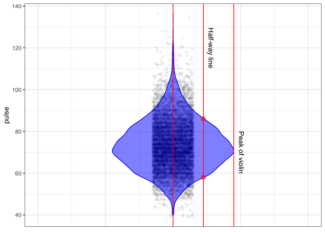
If you have a display of the distribution such as a violin plot or a density plot, there’s another way to find the interval from one standard deviation below the mean to one standard deviation above the mean. First, find the peak of the display of the distribution. Then come down half way from the peak and mark the two points where the display of the distribution touches the half-way line. Those points are pretty close to plus-and-minus one standard deviation from the mean.
Explaining (3) is better done with a picture. The figure below shows values of a variable plotted along with a violin display. One line is drawn at the peak of the violin. The “half-way” line is drawn half of the way from the center of the violin to the peak. The two dots show the points whose vertical position is one standard deviation on either side of the mean.

You might prefer one or the other of these three rules of thumb. Try them out and see which works best for you.
Activity
Open up the center-and-spread Little App. (See footnote1). Using the NHANES data, set the response variable to pulse and leave the explanatory variable at .none.. Set the sample size to n = 1000.
Check the “Density violin” box to turn on the violin plot.
Pick one of the three rules of thumb to estimate the mean and standard deviation.
Write down your estimates of the mean and the standard deviation. . . . . .
Check the “Std. deviation” box to turn on a ruler calibrated in units of the standard deviation.
How close were your estimates in (2) to the actual values displayed by the ruler? . . . . .
Turn off the standard deviation ruler and repeat the above for several variables from the various data frames that come with the Little App. You might want to practice several times to get a hang for how to eyeball each of the intervals in the three rules of thumb.
As you work through different variables, note which ones have a violin corresponding to the bell-shaped normal curve. The rules of thumb work best for variables that have a normal-like distribution.
Write down two variables with a bell-shaped distribution. . . .
Write down at least one variable that does not have a bell-shaped distribution. . . .
Now you’re going to find some variables whose density has specific shapes.
`* Find a variable with a density that has a long trailing tail below the mean, but not above it. (This is called “negatively skewed” or “left skewed.”)
Write down the name of the left skewed variable you found. . . .
`* Find a variable with a density that has a long trailing tail above the mean, but not below it it. (This is called “positively skewed” or “right skewed.”)
Write down the name of the right skewed variable you found. . . .
`* Find a variable for which the density has two peaks. (This is called “bimodal.”
Write down the name of the bimodal variable you found. . . .
Version 0.2, 2019-06-20, Thomas Kinzeler and Danny Kaplan, Word version
