DATA SOURCE: Big data from machine-learning sites

Process

1. Download the ZIP file from the repository
2. UNZIP
3. Read in the data

file_name <- "/Users/kaplan/Downloads/comedy_comparisons/comedy_comparisons.train"
Clips <- readr::read_csv(file_name, col_names = FALSE)
names(Clips) <- c("left", "right", "winner")

What to do

As usual, it isn’t clear what statistically informative concept can be illustrated with these data. It’s necessary to explore and see where the data takes you.

In the end, I decided on a simple-sounding question: Which is the best clip? The answer, as you’ll see, involves balancing the win rate and the number of trials.

Here’s the winner …

Exploring

The data are organized as three variables:

left and right contain ID numbers for videos on YouTube. winner indicates whether the left video or the right video were preferred by the viewer.

Some questions:

1. How many reviews are there? How many videos?

   nrow(Clips)

   ## [1] 912969

   length(unique(c(Clips$left, Clips$right)))

   ## [1] 18474

2. Which is the most preferred video?

   Wins <- 
     Clips %>%
     mutate(video = ifelse(winner == "left", left, right)) %>%
     group_by(video) %>%
     summarize(wins  = n()) %>%
     arrange(desc(wins)) 
   head(Wins)

   ## # A tibble: 6 x 2
   ##   video        wins
   ##   <chr>       <int>
   ## 1 C8IJnUM0yQo 33653
   ## 2 W9y6nwBwwyQ 27708
   ## 3 LLaKkC5U9Po 26273
   ## 4 7zCIRPQ8qWc 21130
   ## 5 YowPM7yZv2U 19894
   ## 6 bOcugYjrvLg 19812

   tail(Wins)

   ## # A tibble: 6 x 2
   ##   video        wins
   ##   <chr>       <int>
   ## 1 zyVaOgXWTk8     1
   ## 2 Zz01eubLEZU     1
   ## 3 zZ6VsVmRub0     1
   ## 4 zzGf8A-s-yo     1
   ## 5 ZZlKQ4m_X3g     1
   ## 6 ZzTF7BQ2Mps     1

But see the section on win rate below.

3. How many contests did each video appear in?

   Lefts <- Clips %>% ungroup() %>% group_by(left) %>% summarize(nleft = n())
   Rights <- Clips %>% ungroup() %>% group_by(right) %>% summarize(nright = n()) 
   Contests <-  Lefts %>%
     inner_join(Rights, by = c(left = "right")) %>%
     mutate(total  =  nleft + nright) %>%
     select(left, total)

4. What’s the win rate? Perhaps insist that the p-value against the null of prob one-half be smaller than 0.001 or 0.0001. Or look at the lower bound of the 95% confidence interval on the number of wins.

   Scores <- Wins %>% inner_join(Contests, by = c(video = "left")) %>%
     mutate(win_rate = wins / total) %>%
     mutate(p_value = 1 - pbinom(wins-1, p = 0.5, size = total )) %>%
     mutate(lower = qbinom(.025,  total, win_rate)) %>%
     mutate(pessimist = lower / total)

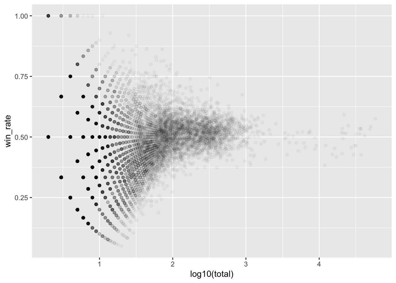
Can you pick which is the best clip?

Plot <- gf_point(win_rate ~ log10(total), data  = Scores, alpha  = 0.03)
Plot

The highest scoring clips are among those with the fewest views.

According to the p-value, which is the best movie?

Scores %>%  
  filter(p_value < 0.0001) %>%
  arrange(desc(pessimist))

## # A tibble: 129 x 7
##    video        wins total win_rate  p_value lower pessimist
##    <chr>       <int> <int>    <dbl>    <dbl> <dbl>     <dbl>
##  1 HE7cxOa9pXg    23    25    0.92  9.72e- 6    20     0.8  
##  2 VCVuWMSd4Nk    62    72    0.861 1.34e-10    56     0.778
##  3 0o-FA5hXaf4    38    44    0.864 4.72e- 7    33     0.75 
##  4 oMgKyG_aAiE    28    32    0.875 9.65e- 6    24     0.75 
##  5 DFMpoEsC-Tc    49    59    0.831 1.35e- 7    43     0.729
##  6 cQzPNT780bs    62    76    0.816 1.16e- 8    55     0.724
##  7 GVaPB-I0d30    49    60    0.817 3.78e- 7    43     0.717
##  8 iaYgMbiR9Rg    24    28    0.857 9.00e- 5    20     0.714
##  9 hED4Tz1JM50    75    94    0.798 2.41e- 9    67     0.713
## 10 3hacWx_k2Oo    56    69    0.812 8.42e- 8    49     0.710
## # … with 119 more rows

Links to be best videos …

Win rates: 92%, 80%