Tidy Data

May 6, 2019

GAISE 2016

Teach statistical thinking.
- Teach statistics as an investigative process of problem-solving and decision-making.
- Give students experience with multivariable thinking.
Focus on conceptual understanding.
Integrate real data with a context and purpose.
Foster active learning.
Use technology to explore concepts and analyze data.
Use assessments to improve and evaluate student learning.

Real data

The StatPREP definition:

captured in the wild: not collected for teaching statistics
appropriate for investigation of a particular question or set of questions
- large enough (think: \(n \ge 1000\))
- rich enough (think: 5 or more variables)

For the moment, put aside the important matters of context and purpose.

Instead, focus on the organization of data in a way that will contribute to

good habits in the workplace
ability to use technology effectively
multivariable thinking

Discipline in presenting data encourages good work habits.

Data organization

Almost all StatPREP participants say they teach little or nothing about organizing data.
- In textbooks, teaching about data focusses on variable types, not organization.
Organizing data properly is critically important for …
- thinking correctly with data
- using real data with technology

Encourage/expose students to “data-base thinking”
- ironically, this is a very mathematical form of thinking, but few mathematicians know about it.
- SQL is the algebra that gets you a job!
- Data base thinking empowers you to explore and present both simple and complex data!

Unruly data

unruly: (adj.) disorderly and disruptive and not amenable to discipline or control

Some Examples

Rules tame unruliness

Always in a “spreadsheet” (ie, rows and columns) fail ✔︎✔︎✔︎
Rows: One row per unit of observation/analysis
- No summaries in data︎
- No other info, e.g. codebook, in spreadsheet fail
- Any subset of rows is a valid data set.
Columns: One column per variable fail
- Always use column names fail
Always codebook fail
- Rows: how cases were selected
- Columns: units, specific questions/protocols/methods
Segregate data collection and data analysis
- Never change the original data as part of the analysis

Note: This sort of tidy/rectangular data is not the only kind of data, but it is an extremely important kind of data and sufficient for introductory courses.

Implications: You need to have a way to distribute such data.

Google spreadsheets, google forms
- Best practices
CSV files
More efficient forms

Operations on Tidy Data

One advantage of tidy data is that it is ammenable to standard, reusable data operations.

Fundamental

summarize / reduce: convert entire data set to 1-row of summary values
- in spreadsheet: often not tidy, summary formulas can be placed in untidy places
- in R: df_stats()
mutate / transform: add new variable
- in spreadsheet: add a new column
- in R: mutate()
filter: remove/ignore rows or columns
- in spreadsheet: “hide” data
- in R: filter()

Superficial

select: remove/ignore columns
- in spreadsheet: “hide” data
- in R: select()
arrange
- in spreadsheet, “sort”. But how do you do this without altering the data?
- in R: arrange()

Profound

group: handle summarize and mutate in a groupwise way
- in spreadsheet: pivot table
- in R: group_by(); formulas (eg, blood_pressure ~ age + sex)
join: bring together data from multiple sources
- in spreadsheet “fusion tables” but will be phased out in Dec. 2019 in terms of SQL operations
spread / gather: change unit of analysis
- in spreadsheet pivot/unpivot
- in R: spread(), gather() [soon to be pivot_wide(), pivot_long()]

Long vs Wide Data

Long

country	continent	year	lifeExp
Afghanistan	Asia	1952	28.801
Afghanistan	Asia	1957	30.332
Afghanistan	Asia	1962	31.997
Afghanistan	Asia	1967	34.020
Afghanistan	Asia	1972	36.088

Wide

country	continent	pop1952	pop1957	pop1962	pop1967	pop1972	pop1977	pop1982	pop1987	pop1992	pop1997	pop2002	pop2007
Afghanistan	Asia	28.801	30.332	31.997	34.020	36.088	38.438	39.854	40.822	41.674	41.763	42.129	43.828
Albania	Europe	55.230	59.280	64.820	66.220	67.690	68.930	70.420	72.000	71.581	72.950	75.651	76.423
Algeria	Africa	43.077	45.685	48.303	51.407	54.518	58.014	61.368	65.799	67.744	69.152	70.994	72.301
Angola	Africa	30.015	31.999	34.000	35.985	37.928	39.483	39.942	39.906	40.647	40.963	41.003	42.731
Argentina	Americas	62.485	64.399	65.142	65.634	67.065	68.481	69.942	70.774	71.868	73.275	74.340	75.320

Quiz

List the many ways in which this “table” violates the conventions for effective data organization.

Variable types

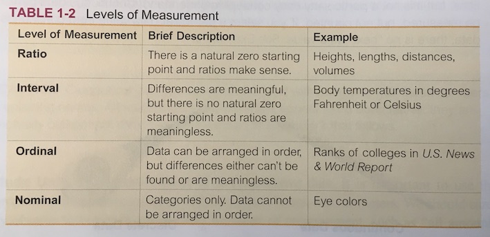
These are often introduced as definitions before the student has any use for them.

In stats book:

Key distinction / minor distinctions

numerical/quantitative: interval, ratio, count, measure, …
categorical: unordered, ordered

Variable types in the wild

Numerical
1. quantities (with dimension and units) –
2. times and dates
3. counts (natural numbers)
4. ~~codes represent discrete levels, not really numerical~~

Categorical
1. “Two-sample” isn’t (usually) two samples
  - one sample, two variables
  - categorical variable identifies the group
2. Summarizing with proportions doesn’t make categrical data numerical
3. fixed vs “random”
  - Fixed: data contains all levels of interest
  - Random: data represents a subset of/sample from levels of interest